MHR, Regular Distributions and Myerson’s Lemma

May 30th, 2011 renatoppl No comments

Monotone Hazard Rate (MHR) distributions and its superclass regular distributions keep appearing in the Mechanism Design literature and this is due to a very good reason: they are the class of distributions for which Myerson’s Optimal Auction is simple and natural. Let’s brief discuss some properties of those distributions. First, two definitions:

Hazard rate of a distribution $f$ : $h(z) = \frac{f(z)}{1-F(z)}$
Myerson virtual value of a distribution $f$ : $\phi(z) = z - \frac{1-F(z)}{f(z)}$

We can interpret the hazard rate in the following way: think of $T \sim f$ as a random variable that indicates the time that a light bulb will take to extinguish. If we are in time $t$ and the light bulb hasn’t extinguished so far, what is the probability it will extinguish in the next $\delta$ time:

$\mathbb{P}[T \leq t+\delta \vert T > t] \approx \frac{f(t) \delta}{1-F(t)}$

We say that a distribution is monotone hazard rate, if $h(z)$ is non-decreasing. This is very natural for light bulbs, for example. Many of the distributions that we are used to are MHR, for example, uniform, exponential and normal. The way that I like to think about MHR distributions is the following: if some distribution has hazard rate $h(z)$ , then it means that $F'(z) = (1-F(z)) h(z)$ . If we define $G(z) = 1-F(z)$ , then $(log G(z))' = \frac{G'(z)}{G(z)} = -h(z)$ , so:

$F(z) = 1-\text{exp}(-\int_0^z h(u) du)$

From this characterization, it is simple to see that the extremal distributions for this class, i.e. the distributions that are in the edge of being MHR and non-MHR are constant hazard rate, which correspond to the exponential distribution $F(z) = 1-e^{-\lambda z}$ for $z \in [0,\infty)$ . They way I like to think about those distributions is that whenever you are able to prove something about the exponential distribution, then you can prove a similar statement about MHR distributions. Consider those three examples:

Example 1: $\mathbb{P}[\phi(z) \geq 0] \geq \frac{1}{e}$ for MHR distributions. This fact is straightforward for the exponential distribution. For the exponential distribution $\phi(z) = z-\lambda^{-1}$ and therefore

$\mathbb{P}[\phi(z) \geq 0] \geq \mathbb{P}[z > \lambda^{-1}] = 1-F(\lambda^{-1}) = e^{-1}$

but the proof for MHR is equally simple: Let $r = \inf \{z; \phi(z) \geq 0\}$ , therefore $r h(r) \leq 1$ .
$P\{ \phi(v) \geq 0\} = P\{ v \geq r \} = 1 - F(r) = e^{-\int_0^r h(u) du} \geq e^{-r h(r)} \geq e^{-1}$

Example 2: Given $z_1, z_2 \sim f$ iid where $f$ is MHR and $v_1 = \max \{z_1, z_2\}$ and $v_2 = \min \{z_1, z_2\}$ , then $\mathbb{E}[v_2] \geq \frac{1}{3} \mathbb{E}[v_1]$ . The proof for the exponential distribution is trivial, and in fact, this is tight for the exponential, the trick is to use the convexity of $z \mapsto \int_0^z h(u) du$ . We use that $\int_0^{2z} h \geq 2 \int_0^z h$ in the following way:

$\mathbb{E} [v_2] = \int_0^\infty (1 - F(z))^2 dz = \int_0^\infty e^{-2 \int_0^z h} dz$

$\geq \int_0^\infty e^{-\int_0^{2z} h} dz= \frac{1}{2} \int_0^\infty 1 - F(z) dz = \frac{1}{2} \mathbb{E} [z]$

Since $\mathbb{E} [v_1 + v_2] = \mathbb{E} [z_1 + z_2] = 2 \mathbb{E} [z]$ , we have that $\mathbb{E}[v_1] = 2 \mathbb{E}[z] - \mathbb{E}[v_2] \leq \frac{3}{2} \mathbb{E}[z]$ . This way, we get: $\mathbb{E}[v_2] \geq \frac{1}{2}\mathbb{E}[z] \geq \frac{1}{2} \cdot \frac{2}{3} \mathbb{E}[v_1] = \frac{1}{3} \mathbb{E}[v_1]$

Example 3: For MHR distributions, there is a simple lemma that relates the virtual value and the real value and this lemma is quite useful in various settings: let $r = \inf \{z; \phi(z) > 0 \}$ , then for $z \geq r$ , $\phi(z) \geq z - r$ . Again, this is tight for exponential distribution. The proof is quite trivial:

$x - \phi(x) = \frac{1-F(x)}{f(x)} \leq \frac{1-F(r)}{f(r)} = r$

Now, MHR distributions are a subclass of regular distributions, which are the distributions for which Myerson’s virtual value $\phi(z)$ is a monotone function. I usually find harder to think about regular distributions than to think about MHR (in fact, I don’t know so many examples that are regular, but not MHR. Here is one, though, called the equal-revenue-distribution. Consider $z \in [1, \infty)$ distributed according to $f(z) = 1/z^2$ . The cumulative distribution is given by $F(z) = 1-1/z$ . The interesting thing of this distribution is that posted prices get the same revenue regardless of the price. For example, if we post any price $r \in [1,\infty)$ , then a customer with valuations $z \sim f$ buys the item if $z > r$ by price $r$ , gettingÂ revenue is $r (1-F(r)) = 1$ . This can be expressed by the fact that $\phi(z) = 0$ . I was a bit puzzled by this fact, because of Myerson’s Lemma:

Myerson Lemma: If a mechanism sells to some player that has valuation $v \sim f$ with probability $x(v)$ when he has value $v$ , then the revenue is $\mathbb{E} [x(v) \phi(v)]$ .

And it seemed that the auctioneers was doomed to get zero revenue, since $\phi(z) = 0$ . For example, suppose we fix some price $r$ and we sell the item if $v \geq r$ by price $r$ . Then it seems that Myerson’s Lemma should go through by a derivation like that (for this special case, although the general proof is quite similar):

$\mathbb{E} [x(v) \phi(v)] = \int_r^\infty \phi(z) f(z) dz = \int_r^\infty z f(z) - (1-F(z)) dz =$

$= \int_r^\infty [ z f(z) - \int_z^\infty f(u) du ] dz = \int_r^\infty z f(z) dz - \int_r^\infty \int_r^u f(u) dz du$

$= r (1-F(r))$

but those don’t seem to match, since one side is zero and the other is 1. The mistake we did above is classic, which is to calculate $\infty - \infty$ . We wrote:

$\mathbb{E}[\phi(v)] = \int_r^\infty z f(z) dz - \int_r^\infty 1-F(z) dz$

but both are infinity! This made me realize that Myerson’s Lemma needs the condition that $\mathbb{E}[z] < \infty$ , which is quite a natural a distribution over valuations of a good. So, one of the bugs of the the equal-revenue-distribution is that $\mathbb{E}[z] = \infty$ . A family that is close to this, but doesn’t suffer this bug is: $f(z) = \frac{\alpha-1}{z^\alpha}$ for $z \in [1,\infty)$ , then $F(z) = 1 - z^{1-\alpha}$ . For $\alpha > 2$ we have $\mathbb{E}[v] < \infty$ , then we get $\phi(z) = \frac{\alpha-2}{\alpha-1} z$ .

Categories: theory Tags: probability, profit maximization

Bimatrix games

May 25th, 2011 renatoppl No comments

This week in Israel is the Workshop on Innovations in Algorithmic Game Theory, which has been a collection of amazing talks and I thought of blogging about something new I learned here. First, Paul Goldberg gave an amazing talk about the Lemke-Howson algorithm and Homotopy Methods. Later, during the poster session Jugal Garg presented the impressive work on an exact algorithm for finding Nash equilibria in rank 1 bimatrix games. Both have in common the use of homotopy, which I found I quite cool idea – and has been present in Game Theory for a while, but I didn’t know about. They also have to do with improving the understanding we have on the Lemke-Howson Algorithm – a (potentially exponential time) algorithm to find Nash equilibrium in 2-person bi-matrix games, but that seems to work pretty well in practice. As always, I though that blogging about it would be a good idea in order to understand those concepts well.

Bimatrix Game and How to compute equilibrium

Bimatrix game is the simplest class of games studied. Basically it is a $2$ player game, with $n$ strategies for player $1$ and $m$ strategies for player 2 which is represented by a pair of $n \times m$ matrices $(A,B)$ . Let $x \in \mathbb{R}_+^n, \Vert x \Vert_1 = 1$ represent a probability distribution that player $1$ assigns to his strategies and $y \in \mathbb{R}_+^m, \Vert y \Vert_1 = 1$ be the same for player $2$ . This way, the players experience utilities:

$[; u_1 (x,y) = x^t A y,Â u_2(x,y) = x^t B y;]$

The best understood class of those games is the one where $A+B = 0$ , called zero-sum games. For this class, computing a Nash equilibrium is very easy and it is given by the famous min-max theorem: player $1$ finds $x$ maximizing $\min_j (x^t A e_j)$ where $e_j$ is the $j$ -th unit vector. Similarly player $2$ finds $y$ maximizing $\min_i (e_i^t B y)$ . Then the pair of strategies obtained is a Nash equilibrium – and this verifying that is not hard.

When $A+B \neq 0$ , the problems gets a lot more complicated. Proving that equilibrium exist can be done using various fixed point theorems, as Brouwer or Kakutani. There is a very simple exponential time algorithm for finding it and the key observation is the following, if $(x,y)$ is a Nash equilibrium then:

$\forall i: x_i = 0 \text{ or } \forall i': e_i^t A y \geq e_{i'}^t A y$

$\forall j: y_j = 0 \text{ or } \forall j': x^t B e_j \geq x^t B e_{j'}$

which means that each strategy for player $i$ is either in the support or is a best response. Proving that is trivial (if some strategy is in the support and is not a best response, then reducing the probability we play it is an improving deviation). Therefore if we just guess the support of $x$ and the support of $y$ we just need to find some strategies with this support satisfying the inequalities above. This can be done using a simple LP. This is clearly not very efficient, since it involves solving $2^{n+m}$ LPs. A still exponential, but a lot more practical method, is:

Lemke-Howson Algorithm

A good overview of the L-H algorithm can be found in those lecture notes or in a more detailed version in third chapter of the AGT book (a pdfÂ can be found in Tim’s website). Here I’ll present a quick overview. The main idea is to define the best-response polytopes $P$ and $Q$ :

$[; P = \{(x,v) \in \mathbb{R}^{n+1} \vert x_i \geq 0, x^t B e_j \leq v; \textbf{1}^t x = 1 \};]$

$[; Q = \{(y,u) \in \mathbb{R}^{m+1} \vert e_i^t A y \leq u, y_j \geq 0; \textbf{1}^t y = 1 \} ;]$

The intuition is that a point $(x,v) \in P$ represents the fact that the payoff $v$ of player $2$ when player $1$ plays $x$ is at least $v$ . We could re-write as $v \geq \max_j x^t B e_j$ .

Each of the polytopes has $m+n$ inequalities and $1$ equality. Given $x$ we define $L(x)$ as the indices of the tight inequalities in $P$ and similarly we define $L(y)$ as the indices of the tight inequalities in $Q$ . The theorem in the previous section can be rephrased as:

$(x,y)$ is Nash equilibrium iff $L(x) \cup L(y) = \{1, 2, \hdots, n+m\}$

So we need to look at points in the polytope below that are fully-labeled. And the way that this is done in L-H is quite ingenious – it is a similar idea that is used by the Simplex Method – walking through the vertices of the polytope looking for the desired vertex. In order to do it, let’s define another polytope:

$[;P' = \{x \in \mathbb{R}^n \vert x_i \geq 0, x^t B e_j \leq 1\} ;]$

$[;Q' = \{y \in \mathbb{R}^m \vert e_i^t A y \leq 1, y_j \geq 0\} ;]$

Note that there is a clear bijection between $P' \setminus 0 \leftrightarrow P$ and $Q' \setminus 0 \leftrightarrow Q$ . This is a projective transformation given by $x \mapsto (\frac{x}{\Vert x \Vert_1},\Vert x \Vert_1)$ . Notice that the labels are preserved by this transformation and the vertex and edges of the polytope are mapped almost 1-1 (except the vertex $0$ ). Notice a couple of details:

1. A vertex in $x \in P'$ corresponds to a point with $n$ labels. A vertex in $y \in Q''$ corresponds to a point with $m$ labels.

2. The point $(0,0)$ corresponds to a fully-labeled point of $P' \times Q'$ , unfortunately this is the only fully-labeled point that doesn’t correspond to a Nash equilibrium.

3. By taking an edge of the polytope (which is define by $n-1$ labels in $P'$ and $m-1$ labels in $Q'$ . We can move between two nodes that are almost fully labeled.

The idea is to consider the set of nodes that are almost fully-labeled: fix some label $k$ and consider all the nodes such that $L(x) \cup L(y) \supseteq \{1 .. k-1, k+1 .. n+m\}$ . Those points are either $(0,0)$ , a Nash equilibrium or they have one duplicated label, since $\vert L(x) \vert + \vert L(y) \vert = n+m$ . An edge is composed of $n+m-1$ labels (no duplicated labels). So, one almost fully-labeled point that is not a Nash or $(0,0)$ is only connected to two other vertices via an edge (which correspond to dropping one of the duplicated labels and following the corresponding edge).

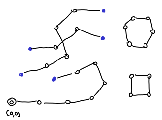
This gives us a topology of the space of Nash equilibria. This tells us a couple of facts: (1) we can find a Nash equilibrium by starting in $(0,0)$ and following the L-H path. In the end of the path, we must find a Nash equilibrium. (ii) If the polytope is not degenerate, then there is an odd number of Nash equilibria and they are connected by L-H edges in the following way:

where the blue dots are the Nash equilibria, the white dots are the almost fully-labeled points and the edges are the L-H edges. The number of Nash equilibria are odd by a simple parity argument.

The classic way in which simplex-like methods walk through the vertices of a polytope is by pivoting. The same way we can implement Lemke-Howson. For an explanation on the implementation, please look at the chapter 3 of the AGT book.

One can ask if we could modify the L-H path following to go through the path faster. Recently, Goldberg, Papadimitriou and Savani proved that finding the Nash equilibrium that L-H outputs is PSPACE-complete. So, in principle, finding this specific equilibrium, seems harder than finding any Nash, which is PPAD-complete.

My current plan is on some other blog posts on Bimatrix games. I wanted to discuss two things: first the homotopy methods and homotopy fixed-point-theorems (which is the heart of the two papers mentioned above) and about new techniques for solving zero-matrix where the strategy space is exponential.

Categories: theory Tags: algorithms, game theory, linear algebra

May 16th, 2011 renatoppl No comments

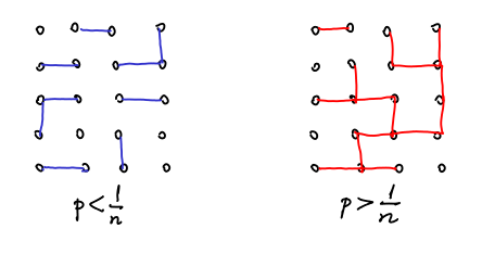
Yesterday I was in a pub with Vasilis Syrgkanis and Elisa Celis and we were discussing about how to calculate the expected size of a connected component in $G(n,p)$ , the ErdÅ‘sâ€“RÃ©nyi model. $G(n,p)$ is the classical random graph obtained by considering $n$ nodes and adding each edge $(i,j)$ independently with probability $p$ . A lot is known about its properties, which very interestingly change qualitatively as the value of $p$ changes relativeto $n$ . For example, for $p <\frac{1}{n}$ then there is no component greater than $O(\log n)$ with high probability. When $p = \frac{c}{n}$ , $c>1$ and $n \rightarrow \infty$ , then the graph has a giant component. All those phenomena are very well studied in the context of probabilistic combinatorics and also in social networks. I remember learning about them in Jon Kleinberg’s Structure of Information Networks class.

So, coming back to our conversation, we were thinking on how to calculate the size of a connected component. Fix some node $u$ in $G(n,p)$ – it doesn’t matter which node, since all nodes are equivalent before we start tossing the random coins. Now, let $C_u$ be the size of the connected component of node $u$ . The question is how to calculate $C(n,p) = \mathbb{E} [C_u]$ .

Recently I’ve been learning MATLAB (actually, I am learning Octave, but it is the same) and I am very amazed by it and impressed about why I haven’t learned it before. It is a programming language that somehow knows exactly how mathematicians think and the syntax is very intuitive. All the operations that you think of performing when doing mathematics, they have implemented. Not that you can’t do that in C++ or Python, in fact, I’ve been doing that all my life, but in Octave, things are so simple. So, I thought this was a nice opportunity for playing a bit with it.

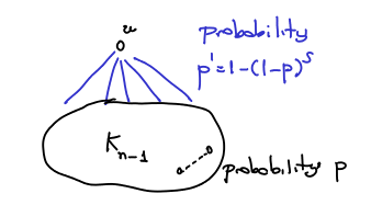
We can calculate $C(n,p)$ using a dynamic programming algorithm in time $O(n^2)$ – well, maybe we can do it more efficiently, but the DP I thought was the following: let’s calculate $\mathcal{C}(n,s,p)$ where it is the expected size of the $u$ -connected component of a random graph with $n$ nodes where the edges between $u$ and other nodes have probability $p' = 1 - (1-p)^s$ and an edge between $v_1$ and $v_2$ have probability $p$ . What we want to compute is $C(n,p) = \mathcal{C}(n,1,p)$ .

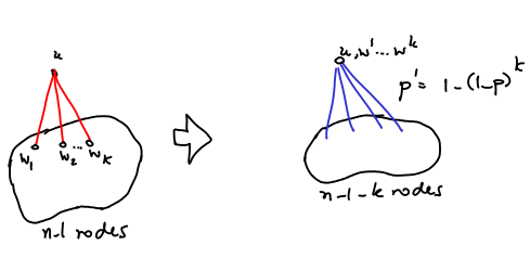
What we can do is to use the Principle of Deferred Decisions,Â and toss the coins for the $n-1$ edges between $u$ and the other nodes. With probability $bin(k,n,p') = {n \choose k} (p')^k (1-‘p)^{n-k}$ , there are $k$ edges between $u$ and the other nodes, say nodes $w_1, \hdots, w_k$ . If we collapse those nodes to $u$ we end up with a graph of $n-k$ nodes and the problem is equivalent to $k$ plus the size of the connected component of $u$ in the collapsed graph.

One difference, however is that the probability that the collapsed node $u$ is connected to a node $v$ of the $n-1-k$ nodes is the probability that at least one of $w_i$ is connected to $v$ , which is $1-(1-p)^k$ . In this way, we can write:

$\mathcal{C}(n,s,p) = 1 \cdot bin(0,n-1,p') + \sum_{k=1}^{n-1} bin(k,n-1,p') [ k + \mathcal{C}(n-k,k,p)]$

where $p' = 1-(1-p)^s$ . Now, we can calculate $C(n,p)$ by using DP, simply by filling an $n \times n$ table. In Octave, we can do it this way:


function component = C(N,p)
  C_table = zeros(N,N);
  for n = 1:N for s =1:N
    C_table(n,s) = binopdf(0,n-1,1-((1-p)^s)) ;
    for k = 1:n-1
      C_table(n,s) += binopdf(k,n-1,1-((1-p)^s)) * (k + C_table(n-k,k));
    end
  end end
  component = C_table(N,1);
endfunction

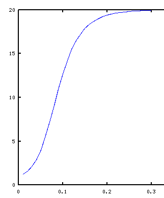
And in fact we can call $C(n,p)$ for say $n = 200$ and $p = 0.01 .. 0.3$ and see how $C(n,p)$ varies. This allows us, for example, to observe the sharp transition that happens before the giant component is formed. The plot we get is:

Categories: theory Tags: probability

Newer Entries Older Entries

Big Red Bits

MHR, Regular Distributions and Myerson’s Lemma

Bimatrix games

DP and the ErdÅ‘sâ€“RÃ©nyi model

ErdÅ‘sâ€“RÃ©nyi model

Recent Posts

Archives

Categories

Comics

Systems Links

Theory Links

Meta