Archive

Archive for April, 2011

Reasoning about Knowledge

April 16th, 2011 No comments

Last week, I went to Petra in Jordan together with Vasilis Syrgkanis and in the road we kept discussing about the Blue-Eyed Islanders Puzzle, posted by Terry Tao on his blog. It is a nice puzzle because it allows us to reflect on how to think about knowledge and how to make statements like “A knows that B knows that C doesn’t know fact F”. My goal in this post is not to discuss about the puzzle itself, but about a framework that allows us to think about it in a structured way. Nevertheless, I strongly recommend the puzzle, first because it is a lot of fun, and second, because it gives a great non-trivial example to think about this kind of thing. But first, a photo from Petra:

And then some references:

I first read Aumann’s classic, which is a very beautiful and short paper — but where I got most intuition (and fun) was reading Chapter 2 of Reasoning About Knowledge.  So, I’ll show here something in between of what Chapter 2 presents and what Geanakoplos’ survey presents (which is also an amazing source).

We want to reason about the world and the first thing we need is a set \Omega representing all possible states the world can take. Each \omega \in \Omega is called a state of the world and completely described the world we are trying to reason about. To illustrate the example, consider the situation where there are n people in a room and each person has a number x_i \in \{0,1\} in his head. Person i can see the number of everyone else, except his. We want to reason about this situation, so a good way to describe the world is to simply define \Omega = \{0,1\}^n of all 0,1-strings. We define an event to be simply a subset of the possible states of the world, i.e., some set E \subseteq \Omega. For example, the even that player 1 has number 0 in his head is simply: E = \{ x \in \Omega; x_1 = 0 \}. We could also think about the event E' that the sum of the numbers is odd, which would be: E' = \{ x \in \Omega; \sum_i x_i \text{ mod } 2 = 1 \}. Now, we need to define what it means for some person to know some event.

For each person i, his knowledge structure is defined by a partition P_i of  \Omega. The rough intuition is that player i is unable to distinguish two elements \omega_1, \omega_2 in the same cell of partition P_i. For each \omega, P_i(\omega) is the cell of partition P_i containing \omega . The way I see knowledge representation is that if \omega is the true state of the world, then person i knows that the true state of the world is some element in P_i(\omega).

Definition: We say that person i knows event E on the state of the world \omega is P_i(\omega) \subseteq E. Therefore, if person i knows event E, the world must be in some state K_i(E) := \{\omega \in \Omega; P_i(\omega) \subseteq E\}.

Above we define the knowledge operator K_i(\cdot). Below, there is a picture in which we represent its action:
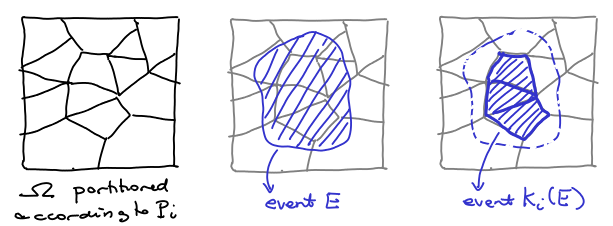
Now, this allows us to represent the fact that person 1 knows that person 2 knows of event E as the event K_1(K_2(E)). Now, the fact the person 1 knows that person 2 doesn’t know that person 1 knows event E can be represented as: K_1(\neg K_2(K_1(E))), where \neg E := \Omega \setminus E.

An equivalent and axiomatic way of defining the knowledge operator is by defining it as an operator K_i: 2^\Omega \rightarrow 2^\Omega such that:

  1. K_i(\Omega) = \Omega
  2. K_i(A) \cap K_i(B) = K_i(A \cap B)
  3. K_i(A) \subseteq A
  4. K_i(K_i(A)) = K_i(A)
  5. \neg K_i(A) = K_i(\neg K_i(A))

Notice that axioms 1-4 define exactly a topology and together with 5 it is a topology that is closed under complement. The last two properties are more interesting: they say that if player i knows something, then he knows that he knows and if the doesn’t know something, he knows that he doesn’t know. Aumann goes ahead and defines the notion of common knowledge:

Definition: We say that an event E is common knowledge at \omega if for any k and for any sequence i(1), \hdots, i(k) where i(j) are players, then \omega \in K_{i(1)} K_{i(2)} \hdots K_{i(k)} E.

Suppose that P' is a partition that is a simultaneous coarsening of P_1, \hdots, P_k, then for all cells C of this partition, either C or \neg C is common knowledge.

An alternative representation is to represent $\Omega$ as nodes in a graph and add an edge between \omega_1 and \omega_2 labeled with i if they are in the same cell of P_i. Now, given the true state of the world \omega \in \Omega, one can easily calculate the smallest event E such that i knows E: this is exactly the states that are reached from \omega just following edges labeled with i, which is easily recognizable as P_i(\omega).

Now, what is the smallest set that 1 knows that 2 knows ? Those are the elements that we can arrive from a path following first an edge labeled 1 and then an edge labeled 2. Extending this reasoning, it is easy to see that the smallest set that is common knowledge at \omega are all the elements reachable from some path in this graph.

More about knowledge representation and reasoning about knowledge in future posts. In any case, I can’t recommend enough the references above.

Categories: theory Tags: ,

Do we believe the Axiom of Choice ?

April 10th, 2011 No comments

Continuing on my series of posts from Israel, I’d like to share some exciting puzzle that I heard today from Omer Tamuz. I’ve learned before about the Axiom of Choice in a Measure Theory class, but never saw a so striking and counter-intuitive application of it. Ok, you might say the Banach–Tarski paradox is a pehaps better example – but since it’s proof is so complicated, it is not as striking as seeing how a simple application of it can generate un-intuitive results. First, let me present two puzzles:

Puzzle #0: There are n+1 people in a line, and each has a 0/1 number on his hat. Each player can look to the numbers of the players in front of him. So, if x_i is the number of player i, then player i knows x_{i+1},\hdots,x_n. Now, from i = 0 \hdots n the players will say his own number. Is there a protocol such that players 1,\hdots,n will get their own number right? (Notice that they hear what the players before him said).

Puzzle #1: Consider the same puzzle with an infinite number of players. I.e. there are x_i; i \in \mathbb{Z}_+ and player i knows x_j for all j > i. Show a protocol for all players, except the first to get the answer right?

Puzzle #2: Still the same setting, but now players don’t hear what the previous player said. Is there a protocol such that only a finite number of players get it wrong ? (notice that it needs to be finite, not bounded).

Puzzle #0 is very easy and the answer is simply parity check. Player 0 could  simply declares y = x_1 \otimes\hdots \otimes x_n where \otimes stands for XOR. Now, player 1 can for example reconstruct x_1 by y \otimes x_2 \otimes \hdots \otimes x_n. Now, player 2 can do the same computation and figure out x_1. Now, he can calculate x_2 = y \otimes x_1 \otimes x_2 \otimes \hdots \otimes x_n and so on… When we move to an infinite number of players, however, we can’t do that anymore because taking the XOR of an infinite number of bits is not well defined. However, we can still can solve Puzzles #1 and #2 if we believe and are willing to accept the Axiom of Choice.

Axiom of Choice: Given a family of sets \{ S_i \}_{i \in I} there is a set \{x_i; i \in I\} such that x_i \in S_i, i.e. a set that takes a representative from each element in the family.

It is used, for example to show that there is no measure \mu : 2^{[0,1)} \rightarrow \mathbb{R} that is shift invariant (say under addition modulo 1) and \mu([0,1)) = 1. The proof goes the following way: define the following equivalence relation on [0,1): x \sim y if x - y \in \mathbb{Q}. Now, consider the family of all the equivalence classes and invoke the Axiom of Choice. Let K be the set obtained. Now, we can write the interval as a disjoint union:

[0,1) = \cup_{x \in \mathbb{Q}} (K+x)

where all operations are modulo 1 and K+x = \{y+x; y \in K\}. Since it is an enumerable union, if such a measure existed, then: \mu([0,1)) = \sum_{x \in \mathbb{Q}} \mu(K+x) = \sum_{x \in \mathbb{Q}} \mu(K) which is either 0 if \mu(K) = 0 or \infty if \mu(K) >0.

This is kinda surprising, but more surprising is how we can use the exact same technique to solve the puzzles: first, let’s solve Puzzle #2: let S be the set of all infinite \{0,1\}-strings and consider the equivalence relation on S such that x \sim y if the strings differ in a finite number of positions. Now, invoke the axiom of choice in the equivalence classes and let S_0 be the set of representatives. Now, if F is the set of all strings with finite number of 1‘s and \otimes the operation such that z = x \otimes z if z_i = x_i \otimes y_i. We can therefore write:

S = \cup_{x \in F} (S_o \otimes x)

Now, a protocol the players could use is to look ahead and since they are seeing an infinite number of bits, they can figure out which equivalence class from S/\sim they the entire string is. Now, they take y \in S_0 the representative of this class and guess y_i. Notice that y will differ from the real string by at most a finite number of bits.

Now, to solve puzzle #1, the player 0 simply looks at x = x_1 x_2 \hdots and figure out the equivalence class he is and let y \in S_0 be the representative of this class. Now, since x and y differ by a finite number of bits, he can simply calculate XOR of x and y (now, since it is a finite number of them, XOR is well defined) and announce it. With this trick, it just becomes like Puzzle #0.

Submodular Allocation Problem

April 6th, 2011 No comments

I am in Israel for the Algorithmic Game Theory Semester in the Center for the Study of Rationality. It is great to both explore Jerusalem and learn about games and algorithms. I think it is a great opportunity to start blogging again. To start, I decided to write about simple and beautiful algorithm by Lehman, Lehman and Nisan on the allocation problem when players have submodular valuations.

Consider a set of m items and n agents. Each agent has a monotone submodular v_i valuation over the items,  i.e., v_i:2^{[m]} \rightarrow \mathbb{R} s.t. v_i(S) + v_i(T) \geq v_i(S \cap T) + v_i(S \cup T) for any subsets S,T of [m] and f(S) \leq f(T) for S \subseteq T. Now, the goal is to partition the items in n sets S_1, \hdots, S_n in order to maximize \sum_i v_i(S_i).

This problem is clearly NP-hard (for example, we can reduce from Maximum Coverage or any similar problem), but is has a very simples Greedy Approximation. The approximation goes as follows: start with all sets being empty, i.e., start with S_i = \emptyset, \forall i then for each item j, find the player i with maximum v_i(j \vert S_i) = v_i(S_i \cup \{j\}) - v_i(S_i) and add j to this player. This is a 2-approximation algorithm. The proof is simple:

Let S_1, \hdots, S_n be the sets returned by the algorithm and O_1, \hdots, O_n the optimal solution. Let also S_i^{<j} = S_i \cap \{1, 2, \hdots, j-1\} and O_i^{<j} = O_i \cap \{1, 2, \hdots, j-1\}. We can write:

\sum_i v_i(S_i) = \sum_i \sum_{j \in S_i} v_i(j \vert S_i^{<j})

if we added j to set S_i it means that v_i(j \vert S_i^{<j}) \geq v_k(j \vert S_k^{<j}) by the Greedy rule. Therefore we can write:

\sum_i v_i(S_i) \geq \sum_k \sum_{j \in O_k} v_k(j \vert S_k^{<j}) \geq \sum_k \sum_{j \in O_k} v_k(j \vert S_k^{<j} \cup O_k^{<j})

where the first inequality follows from the Greedy rule and the second follows from submodularity. Now, we can simply write:

\begin{aligned} \sum_i v_i(S_i) & \geq \frac{1}{2} \sum_i \sum_{j \in S_i} v_i(j \vert S_i^{<j}) + \frac{1}{2} \sum_k \sum_{j \in O_k}  v_k(j \vert S_k^{<j} \cup O_k^{<j}) \\ & \geq \frac{1}{2} \sum_i \sum_{j \in S_i} v_i(j \vert S_i^{<j}  \cup O_i^{<j}) + \frac{1}{2} \sum_k \sum_{j \in O_k}  v_k(j \vert  S_k^{<j} \cup O_k^{<j}) \\ & \geq \frac{1}{2} \sum_i \sum_{j \in S_i \cup O_i} v_i(j \vert S_i^{<j} \cup O_i^{<j}) \\ & = \frac{1}{2} \sum_i v_i(S_i \cup O_i) \geq \frac{1}{2} \sum_i v_i(O_i) \end{aligned}

An improved algorithm was given by Dobzinski and Shapira achieving an 1 -\frac{1}{e} approximation using demand queries – that are used as a separation oracle for a suitable linear program.

Categories: theory Tags: ,