Big Red Bits

This week in Israel is the Workshop on Innovations in Algorithmic Game Theory, which has been a collection of amazing talks and I thought of blogging about something new I learned here. First, Paul Goldberg gave an amazing talk about the Lemke-Howson algorithm and Homotopy Methods. Later, during the poster session Jugal Garg presented the impressive work on an exact algorithm for finding Nash equilibria in rank 1 bimatrix games. Both have in common the use of homotopy, which I found I quite cool idea – and has been present in Game Theory for a while, but I didn’t know about. They also have to do with improving the understanding we have on the Lemke-Howson Algorithm – a (potentially exponential time) algorithm to find Nash equilibrium in 2-person bi-matrix games, but that seems to work pretty well in practice. As always, I though that blogging about it would be a good idea in order to understand those concepts well.

Bimatrix Game and How to compute equilibrium

Bimatrix game is the simplest class of games studied. Basically it is a player game, with strategies for player and strategies for player 2 which is represented by a pair of matrices . Let represent a probability distribution that player assigns to his strategies and be the same for player . This way, the players experience utilities:

The best understood class of those games is the one where , called zero-sum games. For this class, computing a Nash equilibrium is very easy and it is given by the famous min-max theorem: player finds maximizing where is the -th unit vector. Similarly player finds maximizing . Then the pair of strategies obtained is a Nash equilibrium – and this verifying that is not hard.

When , the problems gets a lot more complicated. Proving that equilibrium exist can be done using various fixed point theorems, as Brouwer or Kakutani. There is a very simple exponential time algorithm for finding it and the key observation is the following, if is a Nash equilibrium then:

which means that each strategy for player is either in the support or is a best response. Proving that is trivial (if some strategy is in the support and is not a best response, then reducing the probability we play it is an improving deviation). Therefore if we just guess the support of and the support of we just need to find some strategies with this support satisfying the inequalities above. This can be done using a simple LP. This is clearly not very efficient, since it involves solving LPs. A still exponential, but a lot more practical method, is:

Lemke-Howson Algorithm

A good overview of the L-H algorithm can be found in those lecture notes or in a more detailed version in third chapter of the AGT book (a pdf  can be found in Tim’s website). Here I’ll present a quick overview. The main idea is to define the best-response polytopes and :

The intuition is that a point represents the fact that the payoff of player when player plays is at least . We could re-write as .

Each of the polytopes has inequalities and equality. Given we define as the indices of the tight inequalities in and similarly we define as the indices of the tight inequalities in . The theorem in the previous section can be rephrased as:

is Nash equilibrium iff

So we need to look at points in the polytope below that are fully-labeled. And the way that this is done in L-H is quite ingenious – it is a similar idea that is used by the Simplex Method – walking through the vertices of the polytope looking for the desired vertex. In order to do it, let’s define another polytope:

Note that there is a clear bijection between and . This is a projective transformation given by . Notice that the labels are preserved by this transformation and the vertex and edges of the polytope are mapped almost 1-1 (except the vertex ). Notice a couple of details:

1. A vertex in corresponds to a point with labels. A vertex in corresponds to a point with labels.

2. The point corresponds to a fully-labeled point of , unfortunately this is the only fully-labeled point that doesn’t correspond to a Nash equilibrium.

3. By taking an edge of the polytope (which is define by labels in and labels in . We can move between two nodes that are almost fully labeled.

The idea is to consider the set of nodes that are almost fully-labeled: fix some label and consider all the nodes such that . Those points are either , a Nash equilibrium or they have one duplicated label, since . An edge is composed of labels (no duplicated labels). So, one almost fully-labeled point that is not a Nash or is only connected to two other vertices via an edge (which correspond to dropping one of the duplicated labels and following the corresponding edge).

This gives us a topology of the space of Nash equilibria. This tells us a couple of facts: (1) we can find a Nash equilibrium by starting in and following the L-H path. In the end of the path, we must find a Nash equilibrium. (ii) If the polytope is not degenerate, then there is an odd number of Nash equilibria and they are connected by L-H edges in the following way:

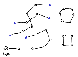
where the blue dots are the Nash equilibria, the white dots are the almost fully-labeled points and the edges are the L-H edges. The number of Nash equilibria are odd by a simple parity argument.

The classic way in which simplex-like methods walk through the vertices of a polytope is by pivoting. The same way we can implement Lemke-Howson. For an explanation on the implementation, please look at the chapter 3 of the AGT book.

One can ask if we could modify the L-H path following to go through the path faster. Recently, Goldberg, Papadimitriou and Savani proved that finding the Nash equilibrium that L-H outputs is PSPACE-complete. So, in principle, finding this specific equilibrium, seems harder than finding any Nash, which is PPAD-complete.

My current plan is on some other blog posts on Bimatrix games. I wanted to discuss two things: first the homotopy methods and homotopy fixed-point-theorems (which is the heart of the two papers mentioned above) and about new techniques for solving zero-matrix where the strategy space is exponential.

I’ve been reading about the Bounded Degree Spanning Tree problem and I thought of writing some of what I am learning here. It illustrates a beautiful techique called Iterated Rounding and uses the combinatorial idea of uncrossing. I’ll try to give a high-level idea of the argument and give references on the details. The first result of this kind was given by Goemans (although there were previous results with weaker guarantees) by Goemans in Minimum Bounded Degree Spanning Trees, but the result based on iterated rounding and a subsequent improvement are due to Singh and Lau in a serie of papers. A main reference is Approximating minimum bounded degree spanning trees to within one of optimal.

The problem of bounded degree spanning tree is as follows: consider a graph with edge weights and we for some nodes a degree bound . We want to find, among the spanning trees for which the degree of is the one with minimum cost. It is clearly a hard problem, since taking all weights equal to and for all nodes is the Hamiltonian Path problem, which is NP-complete. We will get a different kind of approximation. Let OPT be the optimal solution: we will show an algorithm that gives a spanning tree of cost such that each node has degree (this can be improved to with a more sofisticated algorithm, also based on Iterated Rounding).

As always, the first step to design an approximation algorithm is to relax it to an LP. We consider the following LP:

The first constraint expresses that in a spanning tree, there are at most edges, the second prevent the formation of cycles and the third guarantees the degree bounds. For we have the standard Minimal Spanning Tree problem and for this problem the polytope is integral. With the degree bounds, we lose this nice property. We can solve this LP using the Ellipsoid Method. The separation oracle for the is done by a flow computation.

Iterated Rounding

Now, let’s go ahead and solve the LP. It would be great if we had an integral solution: we would be done. It is unfortunately not the case, but we can still hope it is almost integral in some sense: for example, some edges are integral and we can take them to the final solution and recurse the algorithm on a smaller graph. This is not far from truth and that’s the main idea of the iterated rounding. We will show that the support of the optimal solution has some nice structure. Consider the following lemma:

Lemma 1 For any basic solution of the LP, either there is with just one incident edge in the support or there is one such that that at most edges are incident to it.

If we can prove this lemma, we can solve the problem in the following way: we begin with an empty tree: then we solve the LP and look at the support . There are two possibilities according to the lemma:

• If there is one node with just one edge incident to it in the support, we add it to the tree, remove from , decrease , make (the trick is to remove in each iteration edges from that are not in the support. Clearly, removing those edges doesn’t hurt the objective value) and run the algorithm again. Notice that the LP called in the recursion has value less or equal then the actual LP . So if by induction we get a spanning tree respecting the new degree bounds plus two and value less or equal than the new LP value, we can just add and we have a solution with value less or equal than the one of the original LP respecting the degree bounds plus two.
• Otherwise, there is one node that has degree in the support. So, we just remove that degree bound on that vertex (i.e. remove from ), make (again,eliminate the edges not in the support) and run the algorithm again. Clearly, if one node is still in , it has , since there are only three edges in the support, there will be for the rest of the computation, just three edges incident to it, so there will be at most three edges more incident to it. So it will exceed its original by at most .

The algorithm eventually stops, since in each iteration we have less edges or less nodes in and the solution is as desired. The main effort is therefore to prove the lemma. But before, let’s look at the lemma: it is of the following kind: “any basic solution of the LP has some nice properties, which envolve having a not too big (at least in some point) support”. So, it involves proving that the support is not too large. That is our next task as we are trying to prove the lemma. And we will be done with:

Theorem 2 The algorithm described above produces a spanning tree of cost (the LP values and therefore )in which each node has degree .

Bounding the size of the support

We would like now to prove some result like the Lemma above: that in the solution of the LP we have either one with degree in or we have a node in with degree . First, we suppose the opposite, that has all the nodes with degree and all the nodes in have degree . This implies that we have a large number of edges in the support. From the degrees, we know that:

We want to prove that the support of the LP can’t be too large. The first question is: how to estimate the size of the support of a basic solution. The constraints look like that:

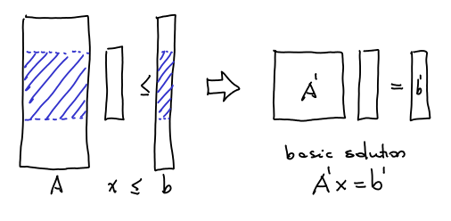
A basic solution can be represented by picking rows of the matrix and making them tight. So, if we have a general LP, we pick some submatrix of which is and the basic solution is just . The lines of matrix can be of three types: they can be , which are corresponding to , that correspond to or corresponding to . There are vectors in total. The size of the support is smaller or equal the number of rows of the form in the basic solution. Therefore the idea to bound the size of the support is to prove that “all basic solutions can be represented by a small number of rows in the form . And this is done using the following:

Lemma 3 Assuming , for any basic solution , there is and a family of sets such that:

1. The restrictions correspondent to and are tight for
2. is an independent set
3. 
4. is a laminar family

The first 3 items are straightfoward properties of basic solutions. The fourth one, means that for two sets , one of three things happen: , or . Now, we based on the previous lemma and in the following result that can be easily proved by induction, we will prove Lemma 1.

Lemma 4 If is a laminar family over the set where each set contains at least elements, then .

Now, the proof of Lemma 1 is easy. Let’s do it and then we come back to prove Lemma 3. Simply see that what contradicts .

Uncrossing argument

And now we arrive in the technical heart of the proof, which is proving Lemma 3. This says that given any basic solution, given any feasible solution, we can write it as a “structured” basic solution. We start with any basic feasible solution. This already satifies (1)-(3), then we need to change that solution to satisfy condition (4) as well. We need to get rid crossing elements, i.e., in the form:

We do that by the means of the:

Lemma 5 (Uncrossing Lemma) If and are intersecting and tight (tight in the sense that their respective constraint is tight), then and are also tight and:

Which corresponds to that picture:

Proof: First, we note that is a supermodular function, i.e.:

We can see that by case analysis. Every edge appearing in the left side appears in the right side with at least the same multiplicity. Notice also that it holds with strict inequality iff there are edges from to . Now, we have:

where the first relation is trivial, the second is by feasibility, the third is by supermodularity and the lastone is by tightness. So, all hold with equality and therefore and are tight. We also proved that:

so there can be no edge from to in and therefore, thinking just of edges in we have:

Uncrossing arguments are found everywhere in combinatorics. Now, we show how the Uncrossing Lemma can be used to prove Lemma 1:

Proof: Let be any basic solution. It can be represented by a pair where and is a family of sets. We will show that the same basic solution can be represented by where is a laminar family and has the same size of .

Let be all sets that are tight under and a maximal laminar family of tights sets in , such that are independent. I claim that .

In fact, suppose , then there are sets of we could add to without violating independence – the problem is that those sets would cross some set. Pick such intersecting fewer possible sets in . The set intersects some . Since both are tight we can use the Uncrossing Lemma and we get:

since , we can’t have simultaneously and in . Let’s consider two cases:

1. , then is in and intersects fewer sets of than , since all sets that intersect in must intersect as well (since no set can cross ).
2. , then is in and intersects fewer sets of than , since all sets that intersect in must intersect .

In either case we have a contradiction, so we proved that . So we can generate all the space of tight sets with a laminar family.

And this finishes the proof. Let’s go over all that we’ve done: we started with an LP and we wanted to prove that the support of each solution was not too large. We wanted that because we wanted to prove that there was one node with degree one in the support or a node in with small () degree. To prove that the degree of the support is small, we show that any basic solution has a representation in terms of a laminar family. Then we use the fact that laminar families can’t be very large families of sets. For that, we use the celebrated Uncrossing Lemma.

Note: Most of this is based on my notes on David Williamson’s Approximation Algorithms class. I spent some time thinking about this algorithm and therefore I decided o post it here.

I was discussing last week with my officemates Hu Fu and Ashwin about the Cayley-Hamilton Theorem. The theorem is the following, given an matrix we can define its characteristic polynomial by . The Cayley-Hamilton Theorem says that . The polynomiale is something like:

so we can just see it as a formal polynomial and think of:

which is an matrix. The theorem says it is the zero matrix. We thought for a while, looked in the Wikipedia, and there there were a few proofs, but not the one-line proof I was looking for. Later, I got this proof that I sent to Hu Fu:

Write the matrix in the basis of its eigenvectors, then we can write where is the diagonal matrix with the eigenvalues in the main diagonal.

and since we have . Now, it is simple to see that:

and therefore:

And that was the one-line proof. One even simpler proof is: let be the eigenvectors, then , so must be since it returns zero for all elements of a basis. Well, I sent that to Hu Fu and he told me the proof had a bug. Not really a bug, but I was proving only for symmetric matrices. More generally, I was proving for diagonalizable matrices. He showed me, for example, the matrix:

which has only one eigenvalue and the the eigenvectors are all of the form for . So, the dimension of the space spanned by the eigenvectors is , less than the dimension of the matrix. This never happens for symmetric matrices, and I guess after some time as a computer scientist, I got used to work only with symmetric matrices for almost everything I use: metrics, quadratic forms, correlation matrices, … but there is more out there then only symmetric matrices. The good news is that this proof is not hard to fix for the general case.

First, it is easy to prove that for each root of the characteristic polynomial there is one eigenvector associated to it (just see that and therefore there must be , so if all the roots are distinct, then there is a basis of eigenvalues, and therefore the matrix is diagonalizable (notice that maybe we will need to use complex eigenvalues, but it is ok). The good thing is that a matrix having two identical eigenvalues is a “coincidence”. We can identify matrices with . The matrices with identical eigenvalues form a zero measure subset of , they are in fact the roots of a polynomial in . This polynomial is the resultant polynomial . Therefore, we proved Cayley-Hamilton theorem in the complement of a zero-measure set in . Since is a continuous function, it extends naturally to all matrices .

We can also interpret that probabilistically: get a matrix where is taken uniformly at random from . Then has with probability all different eigenvalues. So, with probability . Now, just make .

Ok, this proves the Theorem for real and complex matrices, but what about a matrix defined over a general field where we can’t use those continuity arguments. A way to get around it is by using Jordan Canonical Form, which is a generalization of eigenvector decomposition. Not all matrices have eigenvector decomposition, but all matrices over an algebraic closed field can be written in Jordan Canonical Form. Given any there is a matrix so that:

where are blocks of the form:

By the same argument as above, we just need to prove Cayley Hamilton for each block in separate. So we need to prove that . If the block has size , then it is exacly the proof above. If the block is bigger, then we need to look at how does looks like. By inspection:

Tipically, for we have in each row, starting in column the sequence , i.e., . So, we have

If block has size , then has multiplicity in and therefore and therefore, as we wanted to prove.

It turned out not to be a very very short proof, but it is still short, since it uses mostly elementary stuff and the proof is really intuitive in some sense. I took some lessons from that: (i) first it reinforces my idea that, if I need to say something about a matrix, the first thing I do is to look at its eigenvectors decomposition. A lot of Linear Algebra problems are very simple when we consider things in the right basis. Normally the right basis is the eigenvector basis. (ii) not all matrices are diagonalizable. But in those cases, Jordan Canonical Form comes in our help and we can do almost the same as we did with eigenvalue decomposition.