DP and the Erdős–Rényi model
Yesterday I was in a pub with Vasilis Syrgkanis and Elisa Celis and we were discussing about how to calculate the expected size of a connected component in , the Erdős–Rényi model.
is the classical random graph obtained by considering
nodes and adding each edge
independently with probability
. A lot is known about its properties, which very interestingly change qualitatively as the value of
changes relativeto
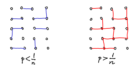
. For example, for
then there is no component greater than
with high probability. When
,
and
, then the graph has a giant component. All those phenomena are very well studied in the context of probabilistic combinatorics and also in social networks. I remember learning about them in Jon Kleinberg’s Structure of Information Networks class.
So, coming back to our conversation, we were thinking on how to calculate the size of a connected component. Fix some node in
– it doesn’t matter which node, since all nodes are equivalent before we start tossing the random coins. Now, let
be the size of the connected component of node
. The question is how to calculate
.
Recently I’ve been learning MATLAB (actually, I am learning Octave, but it is the same) and I am very amazed by it and impressed about why I haven’t learned it before. It is a programming language that somehow knows exactly how mathematicians think and the syntax is very intuitive. All the operations that you think of performing when doing mathematics, they have implemented. Not that you can’t do that in C++ or Python, in fact, I’ve been doing that all my life, but in Octave, things are so simple. So, I thought this was a nice opportunity for playing a bit with it.
We can calculate using a dynamic programming algorithm in time
– well, maybe we can do it more efficiently, but the DP I thought was the following: let’s calculate
where it is the expected size of the
-connected component of a random graph with
nodes where the edges between
and other nodes have probability
and an edge between
and
have probability
. What we want to compute is
.
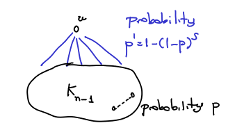
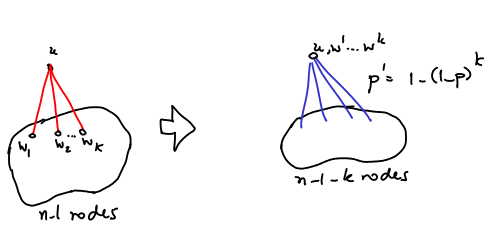
 What we can do is to use the Principle of Deferred Decisions, and toss the coins for the
 edges between
and the other nodes. With probability
, there are
edges between
and the other nodes, say nodes
. If we collapse those nodes to
we end up with a graph of
nodes and the problem is equivalent to
plus the size of the connected component of
in the collapsed graph.
 One difference, however is that the probability that the collapsed node
 is connected to a node
of the
nodes is the probability that at least one of
is connected to
, which is
. In this way, we can write:
where . Now, we can calculate
by using DP, simply by filling an
table. In Octave, we can do it this way:
function component = C(N,p)
  C_table = zeros(N,N);
  for n = 1:N for s =1:N
    C_table(n,s) = binopdf(0,n-1,1-((1-p)^s)) ;
    for k = 1:n-1
      C_table(n,s) += binopdf(k,n-1,1-((1-p)^s)) * (k + C_table(n-k,k));
    end
  end end
  component = C_table(N,1);
endfunction
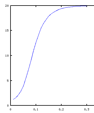
And in fact we can call for say
and
and see how
varies. This allows us, for example, to observe the sharp transition that happens before the giant component is formed. The plot we get is:

